One of the first steps in spatial analysis is to create a neighborhood matrix, that is to say create a relationship/connection between each and (ideally!) every polygon. Why? Well, given that the premise for spatial analysis is that neighboring locations are more similar than far away locations, we need to define what is “near”, a set of neighbors for each location capturing such dependence.
There are many ways to define neighbors, and usually, they are not interchangeable, meaning that one neighborhood definition will capture spatial autocorrelation differently from another.
In R the package spdep allows to create a neighbor matrix according to a wide range of definitions: contiguity, radial distance, graph based, and triangulation (and more). There are 3 main and most used neighbors:
A) Contiguity based of order 1 or higher (most used in social sciences)
B) Distance based
C) Graph based
Install and load the maptools and spdep libraries shapefile from North Carolina counties:
library(maptools)
library(spdep)
NC= readShapePoly(system.file("shapes/sids.shp", package="maptools")[1], IDvar="FIPSNO", proj4string=CRS("+proj=longlat +ellps=clrk66"))
A. Contiguity based relations
are the most used in the presence of irregular polygons with varying shape and surface, since contiguity ignores distance and focuses instead on the location of an area. The function poly2nb allows to create 2 types of contiguity based relations:
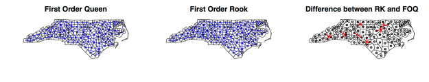
1. First Order Queen Contiguity
FOQ contiguity defines a neighbor when at least one point on the boundary of one polygon is shared with at least one point of its neighbor (common border or corner);
nb.FOQ = poly2nb(NC, queen=TRUE, row.names=NC$FIPSNO)
#row.names refers to the unique names of each polygon
nb.FOQ
## Neighbour list object:
## Number of regions: 100
## Number of nonzero links: 490
## Percentage nonzero weights: 4.9
## Average number of links: 4.9
Calling nb.FOQ you get a summary of the neighbor matrix, including the total number of areas/counties, and average number of links.
2. First Order Rook Contiguity
FOR contiguity does not include corners, only borders, thus comprising only polygons sharing more than one boundary point;
nb.RK = poly2nb(NC, queen=FALSE, row.names=NC$FIPSNO)
nb.RK
## Neighbour list object:
## Number of regions: 100
## Number of nonzero links: 462
## Percentage nonzero weights: 4.62
## Average number of links: 4.62
NB: if there is a region without any link, there will be a message like this:
Neighbour list object:
Number of regions: 910
Number of nonzero links: 4620
Percentage nonzero weights: 0.5924405
Average number of links: 5.391209
10 regions with no links:
1014 3507 3801 8245 9018 10037 22125 30005 390299 390399
where you can identify the regions with no links (1014, 3507,…) using which(…), and in R it is possible to “manually” connect them or change the neighbor matrix so that they can be included (such as graph or distance based neighbors).
Sometimes, it also happens that some polygons that have been retouched (sounds like a blasphemy but it happens a lot with historical maps) may not recognize shared borders. This is when manually setting up neighbors comes in handy (you can’t do that in Geoda).
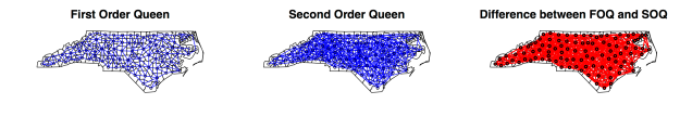
Higher order neighbors are useful when looking at the effect of lags on spatial autocorrelation and in spatial autoregressive models like SAR with a more global spatial autocorrelation:
nb.SRC = nblag(nb.RK,2) #second order rook contiguity
nb.SRC
## [[1]]
## Neighbour list object:
## Number of regions: 100
## Number of nonzero links: 490
## Percentage nonzero weights: 4.9
## Average number of links: 4.9
##
## [[2]]
## Neighbour list object:
## Number of regions: 100
## Number of nonzero links: 868
## Percentage nonzero weights: 8.68
## Average number of links: 8.68
##
## attr(,"call")
## nblag(neighbours = nb.RK, maxlag = 2)
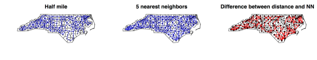
B. Distance based neighbors
DBN defines a set of connections between polygons either based on a (1) defined Euclidean distance between centroids dnearneigh or a certain (2) number of neighbors knn2nb (e.g. 5 nearest neighbors);
coordNC = coordinates(NC) #get centroids coordinates
d05m = dnearneigh(coordNC, 0, 0.5, row.names=NC$FIPSNO)
nb.5NN = knn2nb(knearneigh(coordNC,k=5),row.names=NC$FIPSNO) #set the number of neighbors (here 5)
d05m
## Neighbour list object:
## Number of regions: 100
## Number of nonzero links: 430
## Percentage nonzero weights: 4.3
## Average number of links: 4.3
nb.5NN
## Neighbour list object:
## Number of regions: 100
## Number of nonzero links: 500
## Percentage nonzero weights: 5
## Average number of links: 5
## Non-symmetric neighbours list
a little trick: if you want information on neighbor distances whatever the type of neighborhood may be:
distance = unlist(nbdists(nb.5NN, coordNC))
distance
##   [1] 0.3613728 0.3693554 0.3864847 0.2766561 0.5168459 0.3709748 0.2607982
##   [8] 0.3232974 0.4376632 0.2862144 0.5773310 0.3778483 0.4463538 0.2914539
## ...
## [498] 0.3407192 0.3995114 0.1838115
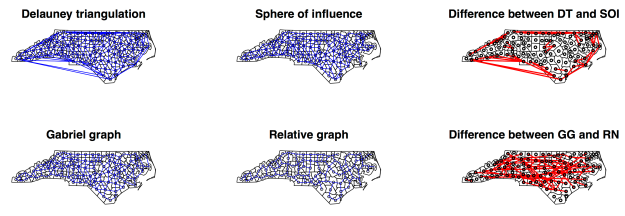
C. Graph based (I’ve never used them, but it’s good to know that they exist)
Delauney triangulation tri2nb constructs neighbors through Voronoi triangles such that each centroid is a triangle node. As a consequence, DT ensures that every polygon has a neighbor, even in presence of islands. The “problem” with this specification is that it treats our area of study as if it were an island itself, without any neighbors (as if North Carolina were an island with no Virginia or South Carolina)… Therefore, distant points that would not be neighbors (such as Cherokee and Brunswick counties) become such;
Gabriel Graph gabrielneigh is a particular case of the DT, where a and b are two neighboring points/centroids if in the circles passing by a and b with diameter ab does not lie any other point/centroid;
Sphere of Influence soi.graph: twopoints a and b are SOI neighbors if the circles centered on a and b, of radius equal to the a and b nearest neighbour distances, intersect twice. It is a sort of Delauney triangulation without the longest connections;
Relative Neighbors relativeneigh is a particular case of GG. A border belongs to RN if the intersection formed by the two circles centered in a and b with radius ab does not contain any other point.
delTrinb = tri2nb(coordNC, row.names=NC$FIPSNO) #delauney triangulation
summary(delTrinb)
## Neighbour list object:
## Number of regions: 100
## Number of nonzero links: 574
## Percentage nonzero weights: 5.74
## Average number of links: 5.74
## Link number distribution:
##
##  2  3  4  5  6  7  8  9 10
##  1  2 13 29 27 22  3  1  2
## 1 least connected region:
## 37039 with 2 links
## 2 most connected regions:
## 37005 37179 with 10 links
GGnb = graph2nb(gabrielneigh(coordNC), row.names=NC$FIPSNO) #gabriel graph
summary(GGnb)
## Neighbour list object:
## Number of regions: 100
## Number of nonzero links: 204
## Percentage nonzero weights: 2.04
## Average number of links: 2.04
## 20 regions with no links:
## 37109 37131 37137 37141 37145 37147 37151 37159 37161 37165 37173 37175 37179 37183 37185 37187 37189 37195 37197 37199
## Non-symmetric neighbours list
## Link number distribution:
##
##  0  1  2  3  4  5  6  7
## 20 27 16 15 13  7  1  1
## 27 least connected regions:
## 37047 37053 37055 37075 37091 37105 37107 37113 37115 37117 37119 37121 37129 37133 37135 37139 37143 37149 37153 37155 37157 37163 37167 37177 37181 37191 37193 with 1 link
## 1 most connected region:
## 37057 with 7 links
SOInb = graph2nb(soi.graph(delTrinb, coordNC), row.names=NC$FIPSNO) #sphere of influence
summary(SOInb)
## Neighbour list object:
## Number of regions: 100
## Number of nonzero links: 470
## Percentage nonzero weights: 4.7
## Average number of links: 4.7
## Link number distribution:
##
##  1  2  3  4  5  6  7  9
##  1  5 12 26 30 15 10  1
## 1 least connected region:
## 37031 with 1 link
## 1 most connected region:
## 37097 with 9 links
RNnb = graph2nb(relativeneigh(coordNC), row.names=NC$FIPSNO) #relative graph
summary(RNnb)
## Neighbour list object:
## Number of regions: 100
## Number of nonzero links: 133
## Percentage nonzero weights: 1.33
## Average number of links: 1.33
## 31 regions with no links:
## 37047 37053 37097 37107 37109 37115 37131 37137 37141 37143 37145 37147 37151 37155 37159 37161 37163 37165 37167 37173 37175 37179 37183 37185 37187 37189 37191 37193 37195 37197 37199
## Non-symmetric neighbours list
## Link number distribution:
##
##  0  1  2  3  4
## 31 30 18 17  4
## 30 least connected regions:
## 37009 37027 37031 37035 37037 37039 37055 37073 37075 37083 37091 37095 37105 37113 37117 37119 37121 37125 37127 37129 37133 37135 37139 37149 37153 37157 37169 37171 37177 37181 with 1 link
## 4 most connected regions:
## 37001 37003 37059 37079 with 4 links
What to do with all this stuff? …
compute and compare global Moran’s I
LISA maps
Variograms and correlograms
…?
